Visualizing Jonathan Dowse’s Vowels

Phonetics
Side Projects
Author

Joey Stanley

Published

December 10, 2023

I’ve seen interactive IPA charts where a single person produces all the sounds. But a couple years ago, I was teaching a Phonetics & Phonology course, and I stumbled upon Jonathan Dowse’s IPA extended chart with audio. In this post, I take his vowels and map their formants.

Note that I tweeted about this on February 7, 2022. I don’t know what the future of X holds, so I thought I’d make this a more permanent home for this plot.

Dowse’s IPA charts

Dowse’s IPA chart is the most detailed one I’ve ever seen. The consonants include many more places of articulation not normally found on the IPA chart, like linguolabial, alveolo-palatal, rounded velar, low uvular, and aryepiglottal. For each one, he uses all the manners that are physically possible, including ones like aspirated stop, affricate, taps, and trills. And for each manner and place, he has voiced and voiceless variants. Not only is the chart itself interesting to look through with all the diacritics and stuff, but he’s got recordings of each consonant in different contexts: [C], [Ca], [aC], and [aCa]. Pretty cool. Further down, he has a whole nother table with “rarer” manners, including lateral fricatives, lateral flaps, fricative trills, implosive, and different kinds of ejectives. It’s pretty interesting to listen to them. He also has a whole table of clicks at eight places of articulation, six manners, and velar and uvular variants of each.

Look, I don’t know enough about phonetics to say whether these are all accurately produced, but it’s impressive that Dowse, who does not appear to have much formal training in linguistics, can produce all these sounds.

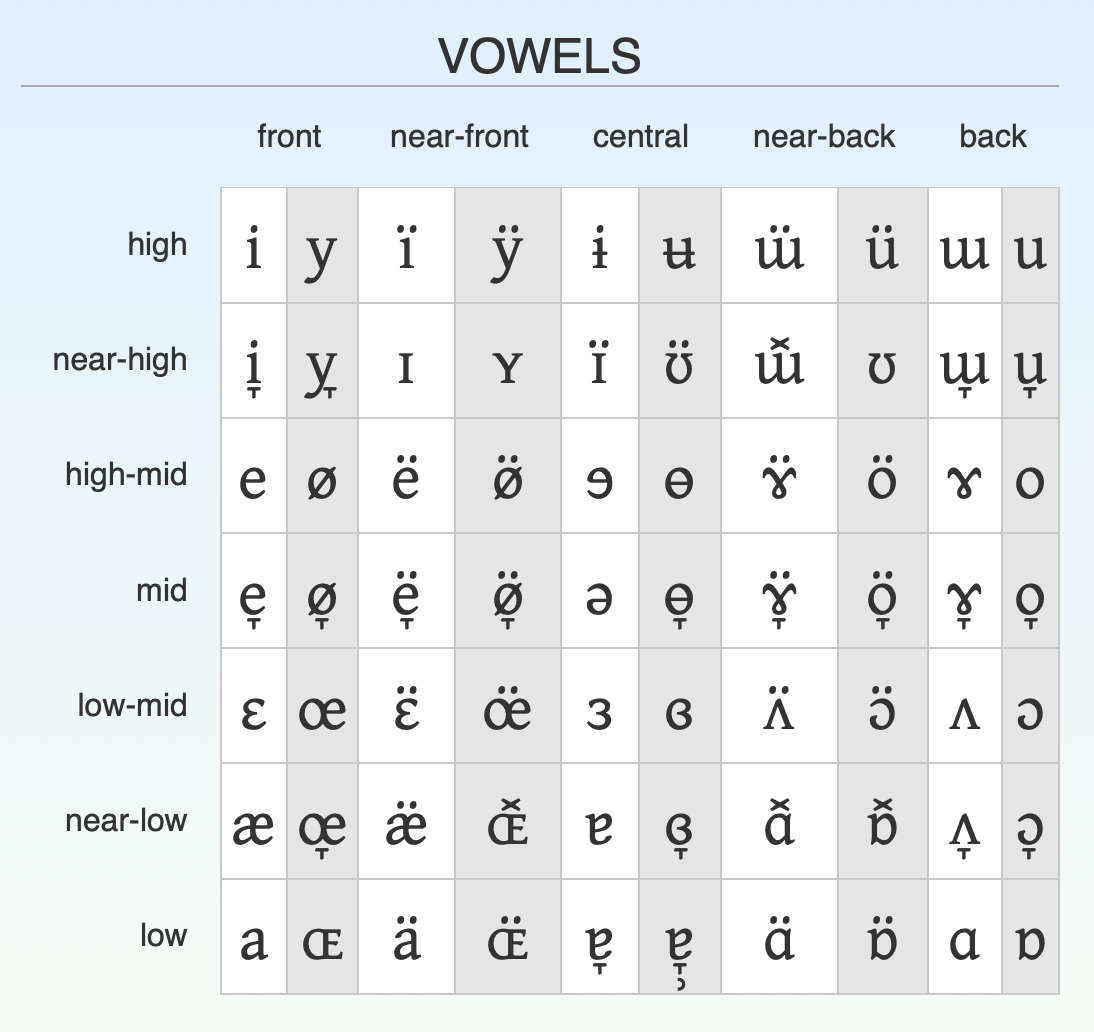
Today’s post is not about the consonants though; it’s about the vowels. His vowel chart is equally extensive. He contrasts five front-to-back distinctions and seven height distinctions, with rounded and unrounded versions of each one. He also has an entirely separate chart showing nasalized versions of all of these.

Jonathan Dowse’s vowel chart

I do know enough about phonetics to be able to look at these vowels. I was curious about how these 70 vowel qualities mapped to the acoustic space. I wanted to see whether these distinctions were all equidistant and whether their distribution in the acoustic space matched this rectangular tabular layout in the chart.

Data Processing

The first step was to download the audio, which I did by just clicking on each one and downloading them one at a time. I then processed them using FastTrack. This produces in a spreadsheet for each vowel produced, with measurements and bandwidths for the first three formants (plus some other measurements) every few milliseconds. Here’s an example from the high front vowel.

library(tidyverse)
library(santoku)

high_front <- read_csv("./csvs/high_front.csv")
knitr::kable(high_front)
time f1 b1 f2 b2 f3 b3 f1p f2p f3p f0 intensity
0.025211 243.0 35.3 2289.2 168.1 3353.6 229.5 219.1 2264.4 3322.6 0.0 53.7
0.027211 245.9 34.9 2201.6 322.6 3356.8 380.5 219.1 2264.9 3322.4 0.0 51.5
0.029211 247.0 44.1 1989.7 553.4 3282.2 640.5 219.1 2265.5 3322.1 0.0 49.4
0.031211 235.4 72.1 1889.2 597.8 3150.0 773.0 219.1 2266.5 3321.5 0.0 48.0
0.033211 208.8 99.9 2035.3 678.2 3253.7 883.0 219.1 2267.7 3320.9 0.0 49.0
0.035211 191.6 96.2 2208.9 525.9 3338.3 574.3 219.2 2269.2 3320.1 0.0 50.1
0.037211 181.0 83.5 2275.7 386.9 3336.5 396.5 219.2 2270.9 3319.2 0.0 52.3
0.039211 173.0 69.6 2305.7 310.2 3332.6 297.6 219.2 2272.9 3318.1 0.0 54.5
0.041211 172.5 58.6 2323.6 242.0 3338.2 243.6 219.3 2275.1 3317.0 0.0 56.6
0.043211 182.6 56.1 2336.8 175.4 3347.3 227.8 219.3 2277.6 3315.7 0.0 58.6
0.045211 196.3 54.5 2348.7 139.8 3348.8 233.9 219.4 2280.3 3314.2 0.0 60.3
0.047211 207.2 48.2 2360.3 131.1 3345.0 244.3 219.4 2283.1 3312.7 0.0 61.9
0.049211 217.3 40.2 2366.6 133.0 3333.5 257.6 219.5 2286.2 3311.1 0.0 63.3
0.051211 227.1 34.3 2363.9 131.5 3316.3 267.5 219.5 2289.5 3309.4 0.0 64.5
0.053211 234.2 30.4 2358.4 120.6 3300.9 263.0 219.6 2292.9 3307.5 0.0 65.4
0.055211 237.1 27.4 2354.8 104.9 3292.8 244.9 219.6 2296.4 3305.6 0.0 66.0
0.057211 237.4 24.6 2353.4 88.3 3291.4 220.6 219.7 2300.1 3303.6 0.0 66.4
0.059211 236.8 21.9 2353.9 73.3 3295.0 196.0 219.8 2303.9 3301.6 0.0 66.5
0.061211 236.1 20.4 2357.3 65.3 3303.0 180.4 219.8 2307.9 3299.5 0.0 66.6
0.063211 235.1 23.4 2367.7 77.1 3310.9 190.6 219.9 2311.9 3297.3 0.0 66.7
0.065211 233.3 31.7 2383.4 109.7 3308.6 217.0 219.9 2316.0 3295.1 0.0 66.9
0.067211 231.9 36.7 2389.0 125.0 3302.6 222.8 220.0 2320.1 3292.8 0.0 67.3
0.069211 231.1 36.1 2386.2 118.2 3300.1 211.3 220.0 2324.3 3290.6 0.0 67.8
0.071211 229.9 33.6 2383.2 108.9 3300.9 199.6 220.1 2328.4 3288.3 0.0 68.2
0.073211 228.0 32.7 2382.5 108.9 3300.4 196.5 220.1 2332.6 3286.0 101.6 68.5
0.075211 226.7 37.0 2383.6 121.4 3291.9 201.8 220.1 2336.8 3283.6 101.7 68.9
0.077211 227.4 42.3 2382.5 128.1 3280.7 202.0 220.2 2341.0 3281.3 101.7 69.2
0.079211 228.4 41.6 2379.4 118.7 3275.4 194.3 220.2 2345.1 3279.0 101.8 69.5
0.081211 227.6 36.0 2378.0 105.1 3275.4 189.0 220.2 2349.1 3276.8 101.8 69.9
0.083211 224.6 30.2 2380.4 100.4 3275.7 201.7 220.2 2353.1 3274.5 101.8 70.2
0.085211 221.3 28.3 2385.8 108.7 3269.8 236.9 220.2 2357.0 3272.3 101.9 70.6
0.087211 220.2 29.6 2388.6 116.3 3261.5 264.0 220.2 2360.8 3270.1 101.9 70.9
0.089211 221.1 29.6 2387.5 111.5 3259.6 263.6 220.2 2364.4 3267.9 102.0 71.1
0.091211 221.7 27.5 2385.5 100.8 3264.8 252.2 220.2 2368.0 3265.9 102.0 71.4
0.093211 220.8 25.7 2384.8 96.7 3272.3 250.8 220.1 2371.4 3263.8 102.1 71.6
0.095211 218.6 26.7 2384.6 103.6 3274.5 262.5 220.1 2374.6 3261.8 102.1 71.8
0.097211 217.4 29.2 2382.4 109.6 3270.4 267.1 220.0 2377.7 3259.9 102.2 72.0
0.099211 217.9 29.2 2378.5 104.7 3269.1 257.5 220.0 2380.6 3258.1 102.2 72.2
0.101211 218.7 26.5 2374.5 96.1 3271.3 246.5 219.9 2383.4 3256.3 102.2 72.3
0.103211 218.2 23.6 2370.8 94.7 3272.5 252.0 219.8 2385.9 3254.6 102.3 72.4
0.105211 216.7 23.4 2368.1 104.2 3266.9 275.4 219.8 2388.3 3253.0 102.3 72.6
0.107211 216.2 24.7 2367.5 110.2 3258.6 287.0 219.7 2390.5 3251.5 102.4 72.7
0.109211 217.2 24.4 2368.4 103.7 3255.9 278.7 219.6 2392.5 3250.0 102.4 72.8
0.111211 218.3 22.3 2369.8 94.3 3255.3 268.6 219.5 2394.3 3248.6 102.4 73.0
0.113211 217.7 20.7 2370.7 94.3 3247.5 282.3 219.3 2395.9 3247.3 102.4 73.1
0.115211 216.0 21.3 2369.8 105.6 3228.5 316.6 219.2 2397.3 3246.1 102.5 73.2
0.117211 215.1 22.8 2368.2 112.7 3213.1 332.0 219.1 2398.5 3245.0 102.5 73.4
0.119211 215.9 22.7 2368.4 106.0 3215.2 321.6 219.0 2399.5 3243.9 102.5 73.5
0.121211 217.0 21.0 2370.6 96.2 3227.2 308.3 218.8 2400.3 3242.9 102.5 73.6
0.123211 216.6 20.4 2373.9 96.0 3238.6 308.4 218.7 2400.9 3242.0 102.5 73.6
0.125211 215.3 22.0 2376.0 108.6 3240.4 316.7 218.5 2401.3 3241.2 102.5 73.7
0.127211 215.0 23.5 2375.1 117.4 3237.6 311.0 218.3 2401.5 3240.4 102.5 73.8
0.129211 216.1 22.8 2373.3 112.0 3239.6 289.1 218.2 2401.6 3239.7 102.4 73.8
0.131211 216.8 21.2 2372.7 102.1 3242.8 267.7 218.0 2401.5 3239.0 102.4 73.9
0.133211 216.0 21.5 2373.7 100.3 3238.3 262.8 217.8 2401.3 3238.4 102.4 73.9
0.135211 214.7 24.8 2375.2 104.5 3225.6 266.6 217.6 2400.9 3237.9 102.4 74.0
0.137211 214.8 27.3 2376.2 100.9 3218.7 256.1 217.4 2400.3 3237.4 102.3 74.0
0.139211 215.9 26.7 2376.9 90.7 3221.4 237.6 217.3 2399.7 3237.0 102.3 74.1
0.141211 216.3 24.3 2377.6 83.1 3227.3 228.6 217.1 2398.9 3236.6 102.2 74.1
0.143211 214.9 23.2 2377.1 86.7 3227.4 241.9 216.9 2398.0 3236.2 102.2 74.1
0.145211 213.3 24.8 2374.6 96.5 3220.0 257.5 216.7 2397.0 3235.9 102.2 74.2
0.147211 213.7 25.8 2371.9 97.1 3216.6 256.6 216.5 2395.9 3235.6 102.1 74.2
0.149211 215.2 24.0 2371.7 89.3 3220.4 248.3 216.3 2394.7 3235.3 102.1 74.2
0.151211 215.7 21.4 2374.4 83.5 3225.9 246.9 216.1 2393.5 3235.0 102.0 74.3
0.153211 214.4 21.2 2379.9 88.3 3226.6 256.1 216.0 2392.2 3234.8 102.0 74.3
0.155211 213.3 23.7 2384.4 98.7 3221.3 259.2 215.8 2390.9 3234.5 101.9 74.3
0.157211 214.1 25.0 2385.0 98.7 3219.3 246.6 215.6 2389.5 3234.3 101.8 74.3
0.159211 215.7 23.6 2384.4 89.1 3223.7 228.9 215.4 2388.2 3234.0 101.8 74.3
0.161211 215.8 21.6 2385.9 81.4 3229.5 220.2 215.3 2386.8 3233.8 101.7 74.3
0.163211 214.0 21.8 2389.7 83.9 3231.0 229.8 215.1 2385.4 3233.5 101.7 74.4
0.165211 212.8 24.1 2392.3 93.4 3225.9 247.9 215.0 2384.1 3233.2 101.6 74.4
0.167211 213.9 24.9 2391.3 95.7 3223.6 257.1 214.8 2382.7 3232.9 101.6 74.4
0.169211 215.7 22.7 2389.5 90.3 3228.7 268.8 214.7 2381.4 3232.6 101.5 74.4
0.171211 215.7 20.0 2389.4 85.4 3241.1 303.4 214.6 2380.1 3232.3 101.5 74.4
0.173211 213.6 19.9 2391.4 87.7 3264.5 359.3 214.4 2378.9 3231.9 101.4 74.4
0.175211 212.3 22.2 2391.3 92.8 3286.5 392.6 214.3 2377.7 3231.5 101.4 74.4
0.177211 213.6 23.4 2388.4 90.6 3285.4 385.8 214.2 2376.6 3231.0 101.3 74.4
0.179211 215.7 22.5 2388.4 82.5 3277.1 353.5 214.1 2375.6 3230.6 101.3 74.4
0.181211 216.1 22.1 2394.2 77.9 3269.0 318.7 214.1 2374.7 3230.1 101.2 74.4
0.183211 214.7 24.5 2401.6 82.8 3255.2 290.2 214.0 2373.8 3229.5 101.2 74.4
0.185211 213.9 28.6 2402.6 91.5 3238.1 262.9 213.9 2373.0 3229.0 101.1 74.4
0.187211 215.1 29.8 2396.0 92.4 3227.8 237.6 213.9 2372.3 3228.4 101.1 74.4
0.189211 216.5 27.4 2389.6 87.0 3226.2 221.8 213.8 2371.7 3227.8 101.0 74.4
0.191211 216.0 24.7 2389.0 85.5 3231.5 230.0 213.8 2371.2 3227.1 101.0 74.4
0.193211 214.0 25.2 2395.5 96.1 3241.3 265.5 213.8 2370.7 3226.4 100.9 74.4
0.195211 213.9 27.5 2401.4 110.0 3248.9 291.4 213.8 2370.4 3225.7 100.9 74.4
0.197211 216.1 27.8 2399.4 111.4 3247.7 279.3 213.8 2370.2 3224.9 100.9 74.4
0.199211 218.1 25.6 2392.9 102.8 3243.2 250.9 213.8 2370.0 3224.2 100.8 74.4
0.201211 217.5 24.0 2388.0 97.4 3237.6 236.7 213.8 2370.0 3223.4 100.8 74.4
0.203211 215.4 25.6 2387.3 102.5 3228.9 247.6 213.8 2370.0 3222.6 100.7 74.4
0.205211 215.0 28.5 2386.9 107.6 3220.8 260.7 213.9 2370.2 3221.8 100.7 74.4
0.207211 216.7 28.4 2383.7 102.9 3217.8 257.6 213.9 2370.4 3220.9 100.6 74.4
0.209211 218.2 25.4 2378.9 93.3 3215.7 248.0 214.0 2370.7 3220.1 100.6 74.4
0.211211 216.9 22.6 2374.3 89.3 3206.7 251.7 214.1 2371.0 3219.2 100.5 74.3
0.213211 213.8 22.8 2371.3 97.0 3186.6 272.9 214.1 2371.4 3218.4 100.5 74.3
0.215211 213.0 24.8 2370.6 104.5 3171.7 282.8 214.2 2371.9 3217.6 100.5 74.3
0.217211 215.1 25.1 2371.5 98.8 3173.5 271.3 214.3 2372.5 3216.8 100.4 74.2
0.219211 216.9 23.4 2372.8 87.9 3182.5 257.3 214.4 2373.1 3215.9 100.4 74.2
0.221211 215.8 22.0 2373.7 83.1 3189.8 264.9 214.5 2373.7 3215.2 100.3 74.1
0.223211 213.2 23.1 2372.8 89.8 3191.7 307.3 214.6 2374.4 3214.4 100.3 74.1
0.225211 213.2 24.6 2370.0 96.1 3194.8 345.5 214.7 2375.1 3213.7 100.3 74.1
0.227211 215.8 24.0 2367.8 90.1 3203.2 333.2 214.8 2375.8 3213.0 100.2 74.1
0.229211 217.7 22.1 2367.2 78.8 3209.6 292.7 215.0 2376.5 3212.3 100.2 74.1
0.231211 216.7 21.4 2367.8 71.3 3210.8 256.6 215.1 2377.2 3211.7 100.2 74.1
0.233211 214.0 23.8 2369.0 74.7 3204.5 257.4 215.2 2378.0 3211.1 100.1 74.1
0.235211 213.7 26.9 2370.1 80.6 3196.6 273.7 215.3 2378.7 3210.5 100.1 74.1
0.237211 216.3 26.9 2370.6 76.8 3197.6 266.8 215.5 2379.4 3210.0 100.1 74.1
0.239211 218.1 24.4 2371.0 67.9 3204.4 245.8 215.6 2380.1 3209.6 100.0 74.1
0.241211 217.0 22.7 2373.3 63.0 3209.0 232.9 215.7 2380.7 3209.2 100.0 74.0
0.243211 214.3 24.6 2379.2 66.6 3205.5 237.7 215.8 2381.3 3208.9 100.0 74.0
0.245211 214.2 27.9 2384.6 71.9 3198.6 248.4 216.0 2381.9 3208.7 100.0 74.0
0.247211 216.9 27.7 2385.0 71.7 3202.8 257.2 216.1 2382.4 3208.5 100.0 74.0
0.249211 218.7 24.1 2381.3 69.5 3219.3 271.9 216.2 2382.9 3208.3 99.9 74.0
0.251211 217.5 21.5 2375.5 71.0 3234.6 287.3 216.3 2383.3 3208.3 99.9 74.0
0.253211 214.9 22.7 2369.4 80.3 3234.3 285.8 216.5 2383.6 3208.3 99.9 74.0
0.255211 214.6 25.6 2364.8 90.6 3226.7 270.4 216.6 2383.9 3208.4 99.9 74.0
0.257211 217.2 26.0 2364.6 88.4 3224.1 248.3 216.7 2384.1 3208.5 99.9 74.0
0.259211 219.1 23.9 2367.9 79.0 3225.2 235.4 216.8 2384.2 3208.7 99.9 74.0
0.261211 217.8 22.1 2373.0 74.1 3224.1 255.8 216.9 2384.3 3209.0 99.9 73.9
0.263211 214.6 23.0 2377.5 79.3 3212.6 324.7 217.0 2384.3 3209.3 99.9 73.9
0.265211 214.1 24.9 2378.2 85.1 3193.5 381.6 217.1 2384.2 3209.7 99.9 73.9
0.267211 216.7 24.8 2377.4 80.0 3189.2 373.0 217.2 2384.0 3210.2 99.9 73.9
0.269211 218.8 23.0 2378.3 69.5 3196.5 336.3 217.3 2383.7 3210.7 99.9 73.9
0.271211 217.8 22.6 2380.8 62.9 3201.5 304.9 217.4 2383.4 3211.3 99.9 73.8
0.273211 214.8 25.8 2382.1 65.2 3194.4 286.6 217.4 2383.0 3211.9 99.9 73.8
0.275211 213.9 29.6 2380.0 70.6 3184.4 272.8 217.5 2382.5 3212.6 100.0 73.8
0.277211 216.0 29.8 2377.0 70.9 3186.8 259.9 217.6 2381.9 3213.3 100.0 73.7
0.279211 217.9 26.6 2376.2 67.2 3199.4 257.5 217.6 2381.3 3214.1 100.0 73.7
0.281211 217.0 23.7 2376.7 67.4 3215.1 278.9 217.7 2380.6 3214.8 100.0 73.7
0.283211 214.3 24.2 2375.1 77.7 3228.2 326.4 217.7 2379.8 3215.7 100.0 73.7
0.285211 214.0 26.0 2369.1 91.7 3233.3 365.9 217.8 2379.0 3216.5 100.0 73.7
0.287211 216.6 25.3 2363.7 94.6 3237.2 368.5 217.8 2378.2 3217.4 100.0 73.7
0.289211 218.6 22.7 2363.4 89.7 3249.1 363.7 217.8 2377.2 3218.3 100.1 73.7
0.291211 217.8 21.0 2367.5 88.0 3269.5 378.6 217.9 2376.3 3219.2 100.1 73.7
0.293211 215.1 22.6 2372.6 93.8 3284.9 402.5 217.9 2375.3 3220.1 100.1 73.7
0.295211 214.6 25.1 2373.5 98.7 3281.4 411.3 217.9 2374.2 3221.0 100.1 73.7
0.297211 216.8 25.2 2371.1 95.2 3269.0 384.6 217.9 2373.2 3222.0 100.1 73.7
0.299211 218.7 23.3 2368.8 87.9 3255.1 334.8 217.9 2372.1 3222.9 100.1 73.7
0.301211 217.8 22.7 2368.0 84.7 3239.2 281.0 217.9 2371.0 3223.7 100.1 73.8
0.303211 215.1 25.8 2368.2 86.9 3219.0 232.6 217.9 2369.9 3224.6 100.1 73.8
0.305211 214.6 30.3 2367.5 84.4 3203.6 195.5 217.9 2368.8 3225.5 100.1 73.8
0.307211 216.9 31.2 2366.3 75.6 3200.0 169.4 217.9 2367.7 3226.3 100.1 73.8
0.309211 218.8 28.7 2365.6 67.7 3201.3 150.2 217.9 2366.6 3227.1 100.1 73.8
0.311211 217.8 26.8 2366.8 68.2 3200.1 140.7 217.9 2365.6 3227.8 100.1 73.8
0.313211 215.0 28.3 2370.2 81.0 3195.6 144.4 217.9 2364.5 3228.5 100.1 73.8
0.315211 214.5 30.6 2372.9 93.0 3194.3 151.1 217.8 2363.5 3229.2 100.1 73.8
0.317211 216.8 29.4 2372.4 91.8 3199.2 154.0 217.8 2362.5 3229.8 100.0 73.8
0.319211 218.8 25.6 2370.8 84.8 3208.6 158.8 217.8 2361.6 3230.3 100.0 73.8
0.321211 218.1 23.2 2370.8 83.1 3218.4 172.5 217.8 2360.7 3230.8 100.0 73.7
0.323211 215.5 24.8 2373.2 91.7 3222.0 196.7 217.8 2359.9 3231.2 100.0 73.7
0.325211 214.8 27.6 2373.8 102.7 3217.8 224.1 217.7 2359.1 3231.6 99.9 73.7
0.327211 216.9 27.2 2371.3 101.7 3218.2 239.1 217.7 2358.3 3231.9 99.9 73.7
0.329211 219.0 24.4 2369.7 91.8 3226.7 242.6 217.7 2357.6 3232.2 99.8 73.7
0.331211 218.6 23.2 2372.6 87.1 3240.6 247.0 217.7 2357.0 3232.4 99.8 73.6
0.333211 216.2 26.1 2379.5 99.1 3250.0 255.0 217.6 2356.5 3232.5 99.7 73.6
0.335211 215.4 30.2 2385.2 120.6 3244.8 249.6 217.6 2356.0 3232.5 99.6 73.6
0.337211 217.4 31.0 2385.1 128.5 3233.9 221.1 217.6 2355.6 3232.5 99.6 73.5
0.339211 219.7 29.1 2381.9 119.3 3227.9 187.7 217.6 2355.2 3232.4 99.5 73.4
0.341211 220.0 28.5 2379.1 109.8 3228.9 169.9 217.6 2354.9 3232.3 99.4 73.4
0.343211 218.5 32.4 2377.1 113.6 3233.4 180.1 217.5 2354.7 3232.1 99.3 73.3
0.345211 218.0 37.2 2373.6 125.7 3237.6 206.3 217.5 2354.6 3231.8 99.3 73.2
0.347211 219.6 36.7 2369.3 128.6 3240.2 212.3 217.5 2354.5 3231.5 99.2 73.1
0.349211 221.5 32.4 2366.5 121.4 3241.6 198.9 217.5 2354.5 3231.1 99.1 73.0
0.351211 221.5 30.0 2364.0 116.9 3242.1 190.2 217.5 2354.5 3230.7 99.0 72.9
0.353211 219.2 32.9 2357.0 125.7 3243.6 209.6 217.4 2354.6 3230.2 99.0 72.8
0.355211 217.5 37.6 2346.3 135.7 3246.8 249.6 217.4 2354.8 3229.7 98.9 72.7
0.357211 218.6 37.6 2339.6 133.0 3251.3 275.8 217.4 2355.0 3229.2 98.8 72.6
0.359211 221.1 33.7 2338.0 124.8 3254.1 278.1 217.4 2355.2 3228.6 98.7 72.5
0.361211 222.5 32.2 2338.1 119.8 3251.1 269.0 217.4 2355.6 3227.9 98.7 72.4
0.363211 221.7 37.3 2335.5 117.9 3240.9 262.0 217.4 2355.9 3227.3 98.6 72.3
0.365211 220.8 44.4 2330.9 110.8 3228.2 262.0 217.4 2356.3 3226.6 98.6 72.2
0.367211 221.9 45.4 2328.6 96.5 3215.1 256.1 217.4 2356.7 3225.9 98.5 72.1
0.369211 224.5 39.4 2330.1 82.5 3204.6 239.4 217.4 2357.2 3225.2 98.5 71.9
0.371211 226.3 32.8 2334.5 75.6 3196.7 219.3 217.4 2357.6 3224.5 98.5 71.8
0.373211 225.5 32.0 2340.0 78.7 3189.4 194.3 217.4 2358.1 3223.8 98.5 71.6
0.375211 223.2 36.7 2343.4 87.4 3186.3 169.8 217.4 2358.6 3223.1 98.5 71.4
0.377211 223.0 39.5 2343.8 89.1 3188.0 148.7 217.4 2359.1 3222.4 98.5 71.2
0.379211 225.3 36.9 2343.4 83.3 3192.2 131.7 217.4 2359.6 3221.7 98.5 71.0
0.381211 227.6 32.8 2343.2 80.5 3195.4 127.5 217.4 2360.1 3221.0 98.5 70.7
0.383211 226.9 32.8 2342.0 95.4 3190.2 155.1 217.4 2360.6 3220.3 98.5 70.5
0.385211 223.0 39.6 2339.8 124.2 3173.0 196.8 217.4 2361.1 3219.7 98.6 70.2
0.387211 220.2 46.7 2339.2 136.8 3164.8 207.9 217.4 2361.5 3219.1 98.6 69.9
0.389211 220.4 47.4 2341.0 131.2 3171.5 198.5 217.4 2361.9 3218.6 98.7 69.6
0.391211 221.1 44.1 2344.3 122.2 3186.6 188.3 217.4 2362.3 3218.1 98.8 69.1
0.393211 218.1 42.0 2349.5 121.2 3209.6 192.6 217.4 2362.7 3217.6 98.8 68.7
0.395211 208.5 47.6 2361.8 135.7 3252.0 225.9 217.4 2363.1 3217.2 98.9 68.2
0.397211 196.3 65.9 2384.7 149.5 3320.3 267.2 217.4 2363.4 3216.8 99.0 67.7
0.399211 188.3 90.3 2398.8 149.3 3358.3 285.7 217.4 2363.6 3216.5 99.0 67.3
0.401211 186.2 109.2 2396.8 169.2 3327.6 310.2 217.4 2363.8 3216.2 99.1 67.0
0.403211 193.1 118.2 2385.1 216.4 3256.3 308.1 217.4 2364.0 3216.0 99.2 66.9
0.405211 210.6 114.3 2377.0 244.9 3200.5 271.1 217.4 2364.1 3215.9 99.3 67.0
0.407211 227.8 109.7 2384.9 213.9 3173.5 233.3 217.4 2364.2 3215.8 99.4 67.1
0.409211 237.6 116.6 2397.5 162.6 3158.1 202.7 217.4 2364.2 3215.8 99.4 67.3

This is more information than I need, especially since Dowse tries to say the vowels as monophthongally as he can. But we can take a look at the trajectories in just a sec. 

So, I want to plot the midpoints of all vowels at once. Since each is stored in a separate spreadsheet, I’ll use Sys.glob to get the paths to all those spreadsheets and map the read_csv function onto all of those paths. Since the vowel quality is stored in the filename itself (i.e., “high_front.csv”), I’ll strip away the path and the extension to leave just that filename and use it as the name of the vowel itself. Finally, I’ll take all those spreadsheets and combine them into one big one with bind_rows and unnest.

vowels_raw <- tibble(vowel = Sys.glob("./csvs/*.csv")) %>%
  mutate(data = map(vowel, read_csv, show_col_types = FALSE),
         vowel = str_remove_all(vowel, "./csvs/"),
         vowel = str_remove_all(vowel, ".csv")) %>%
  bind_rows() %>%
  unnest(data) %>%
  print()
# A tibble: 14,772 × 13
   vowel        time    f1    b1    f2    b2    f3    b3   f1p   f2p   f3p    f0
   <chr>       <dbl> <dbl> <dbl> <dbl> <dbl> <dbl> <dbl> <dbl> <dbl> <dbl> <dbl>
 1 high-mid_… 0.0252  478.  90    918. 122.  2683.  324   423   863. 2696.  107 
 2 high-mid_… 0.0272  476.  77.7  917. 100.  2689.  303.  423.  863. 2696.  107.
 3 high-mid_… 0.0292  470.  71    914.  82.7 2695.  291.  424.  863. 2697.  107.
 4 high-mid_… 0.0312  460.  72.9  908.  77.5 2692.  308.  424.  863. 2698.  107.
 5 high-mid_… 0.0332  451.  78.9  901.  86.2 2680.  337.  425   864. 2700.  107.
 6 high-mid_… 0.0352  450   79    895.  96.9 2675.  336.  426.  864. 2701.  106.
 7 high-mid_… 0.0372  453.  74.6  891.  97.4 2685.  308.  427.  865. 2703.  106.
 8 high-mid_… 0.0392  452.  73.7  887.  92.3 2703.  284.  428.  865. 2705.  106.
 9 high-mid_… 0.0412  448.  81.5  880   94.6 2723.  280.  429.  866  2708.  106.
10 high-mid_… 0.0432  446.  89.6  873. 104.  2740.  284.  431.  867. 2710.  106 
# ℹ 14,762 more rows
# ℹ 1 more variable: intensity <dbl>

This results in a spreadsheet with 14,772 rows, each representing a set of formant measurements at a particular point in time across all 70 recordings. Kind of a lot of data, considering it’s only 70 vowels, but that’s the kind of resolution FastTrack can give you.

Okay, so for the purposes of the plot, I need to create a spreadsheet that is just the metadata about the vowel itself. In Step 1, I take that monster dataframe and just keep the name of the vowel (i.e. “high-mid_back-unrounded”) and only keep unique values. I then split that name up into its three parts (height, backness, and rounded) using separate. In Step 2, I then modify each one of those a little bit. I turn rounded into a boolean instead of a string. Then I turn height and backness into factors and set what order they should be in. Finally, I create a marked column to indicate whether a front vowel is rounded or a back vowel is unrounded—I felt like this might be handy to create a visual of the unmarked vowels. For Step 3, I add the IPA symbols to it. There’s no shortcut: I just had to put the symbols in one at a time based on what the chart showed.

vowels_meta <- vowels_raw %>%
  
  # Step 1: split the vowel name up
  distinct(vowel) %>%
  separate(vowel, c("height", "backness", "rounded"), sep = "_", fill = "right", remove = FALSE) %>%
  
  # Step 2: modify those attributes
  mutate(rounded  = case_when(rounded == "rounded" ~ TRUE,
                             is.na(rounded) ~ FALSE),
         height   = factor(height,   levels = c("high", "near-high", "high-mid", "mid", "low-mid", "near-low", "low")),
         backness = factor(backness, levels = c("front", "near-front", "central", "near-back", "back")),
         marked = case_when(backness %in% c("near-back", "back") & !rounded ~ TRUE,
                            backness %in% c("front", "near-front", "central") & rounded ~  TRUE,
                            TRUE ~ FALSE)) %>%
  
  # Step 3: add IPA
  arrange(height, backness, rounded) %>%
    mutate(ipa = c("i", "y", "ï", "ÿ", "ɨ", "u̶", "ɯ̈", "ü", "ɯ", "u",
                   "i̞", "y̙̞", "ɪ", "ʏ", "ɪ̈", "ʊ̈", "ɯ̽", "ʊ", "ɯ̞", "u̞",
                   "e", "ø", "ë", "ø̈", "ɘ", "ɵ", "ɤ̈", "ö", "ɤ", "o",
                   "e̞", "ø̞", "ë̞", "ø̞̈", "ə", "ɵ̘", "ɤ̞̈", "ö̞", "ɤ̞", "o̞",
                   "ɛ", "œ", "ɛ̈", "œ̈", "ɜ", "ɞ", "ʌ̈", "ɔ̈", "ʌ", "ɔ",
                   "æ", "œ̞", "æ̈", "ɶ̽", "ɐ", "ɞ̞", "ɑ̽", "ɒ̽", "ʌ̞", "ɔ̞",
                   "a", "ɶ", "ä", "ɶ̈", "ɐ̞", "ɐ̞̹", "ɑ̈", "ɒ̈", "ɑ", "ɒ")) %>%

  print()
# A tibble: 70 × 6
   vowel                   height backness   rounded marked ipa  
   <chr>                   <fct>  <fct>      <lgl>   <lgl>  <chr>
 1 high_front              high   front      FALSE   FALSE  i    
 2 high_front_rounded      high   front      TRUE    TRUE   y    
 3 high_near-front         high   near-front FALSE   FALSE  ï    
 4 high_near-front_rounded high   near-front TRUE    TRUE   ÿ    
 5 high_central            high   central    FALSE   FALSE  ɨ    
 6 high_central_rounded    high   central    TRUE    TRUE   u̶    
 7 high_near-back          high   near-back  FALSE   TRUE   ɯ̈    
 8 high_near-back_rounded  high   near-back  TRUE    FALSE  ü    
 9 high_back               high   back       FALSE   TRUE   ɯ    
10 high_back_rounded       high   back       TRUE    FALSE  u    
# ℹ 60 more rows

Okay, so now I have a dataframe that has the name of the vowel from the filename, and then some metadata about that vowel.

Now let’s go back and process that acoustic data. I start by taking the raw data and just keeping the formants. Having like 170 timepoints for each vowel is fine, but when visualizing such data, the odds of getting a wonky one are higher and it’ll ruin the whole plot. Here’s [i]. You can see that most of the formants are pretty stable. But towards the beginning and end, things get weird and they distract from the good data.

ggplot(high_front, aes(f2, f1, color = time)) + 
  geom_path() + 
  scale_x_reverse() + 
  scale_y_reverse() +
  theme_minimal()

What I’ll do then is take all this high resolution temporal data and make it lower resolution. What I found works is to bin the times into about 10 bins and then take the median within each one. I’ll do this by first normalizing the time so that the onset starts at t = 0. That new version of time is now time_diff. I’ll then normalize the time by converting it into percent duration, so that the onset is at 0 and the offset is at 1, with the midpoint at 0.5. That is now in percent. This makes it easier to then slice the data into 10 parts using the santoku::kiru function. For each of those 10 chunks, I can then get the median F1, F2, and F3 measurements.

high_front_summarized <- high_front %>%
  mutate(time_diff = time - min(time),
         percent = time_diff / max(time_diff),
         time_cut = kiru(percent,
                         breaks = seq(0, 1, 0.1),
                         labels = 1:10)) %>%
  summarize(across(c(f1, f2, f3), median), .by = c(time_cut)) %>%
  print()
# A tibble: 10 × 4
   time_cut    f1    f2    f3
   <fct>    <dbl> <dbl> <dbl>
 1 1         231. 2343. 3324.
 2 2         225. 2383. 3275.
 3 3         216. 2371. 3239.
 4 4         214. 2385  3227.
 5 5         216. 2389. 3230.
 6 6         216. 2371  3204.
 7 7         217. 2376. 3215.
 8 8         217. 2371. 3218.
 9 9         220. 2364  3241.
10 10        222. 2344. 3191.

I can plot this new lower-resolution version of the data, and you can see it’s much tighter because the extreme outliers were lost. I’ll add the original data in gray to provide some context.

ggplot(high_front_summarized, aes(f2, f1)) + 
  geom_path(data = high_front, color = "gray80") +
  geom_path() + 
  scale_x_reverse() + 
  scale_y_reverse() +
  theme_minimal()

Okay great. So, that worked for one vowel. Let’s do that for all vowels. The code is the same, except I’m grouping things by vowel. This results in trajs dataframe (for “trajectories”). We’ll look at that in just a second.

trajs <- vowels_raw %>%
  select(vowel, time, f1, f2, f3) %>%
  mutate(time_diff = time - min(time),
         percent = time_diff / max(time_diff),
         time_cut = kiru(percent,
                         breaks = seq(0, 1, 0.1),
                         labels = 1:10),
         .by = vowel) %>%
  summarize(across(c(f1, f2, f3), median), .by = c(vowel, time_cut)) %>%
  print()
# A tibble: 700 × 5
   vowel         time_cut    f1    f2    f3
   <chr>         <fct>    <dbl> <dbl> <dbl>
 1 high-mid_back 1         448.  872. 2745.
 2 high-mid_back 2         431.  835. 2747 
 3 high-mid_back 3         422.  873. 2803.
 4 high-mid_back 4         422.  874  2834.
 5 high-mid_back 5         426.  842. 2789.
 6 high-mid_back 6         416.  844. 2838.
 7 high-mid_back 7         427.  854. 2914.
 8 high-mid_back 8         430.  903. 2874.
 9 high-mid_back 9         404.  966. 3011.
10 high-mid_back 10        967. 1639. 3047 
# ℹ 690 more rows

For now, let’s look at the midpoints. You may have noticed in the high front plot above that the middle 50% or so of the vowel was indeed quite monophthongal with very little formant change. I’ll assume that’s the case for all the vowels. So I’ll take the middle few bins and take the median measurement for each one. That’ll give me a new midpoints dataset.

midpoints <- trajs %>%
  
  # Get the middle few bins and find the median
  filter(time_cut %in% 3:7) %>%
  summarize(across(c(f1, f2, f3), median), .by = vowel) %>%
  
  # Add the vowel metadata back in.
  left_join(vowels_meta, by = "vowel") %>%
  print()
# A tibble: 70 × 9
   vowel                     f1    f2    f3 height backness rounded marked ipa  
   <chr>                  <dbl> <dbl> <dbl> <fct>  <fct>    <lgl>   <lgl>  <chr>
 1 high-mid_back           422.  854. 2834. high-… back     FALSE   TRUE   ɤ    
 2 high-mid_back_rounded   408.  522. 2583. high-… back     TRUE    FALSE  o    
 3 high-mid_central        414. 1670. 2316. high-… central  FALSE   FALSE  ɘ    
 4 high-mid_central_roun…  420.  979. 2322. high-… central  TRUE    TRUE   ɵ    
 5 high-mid_front          416. 2237. 2911. high-… front    FALSE   FALSE  e    
 6 high-mid_front_rounded  346. 2050. 2596. high-… front    TRUE    TRUE   ø    
 7 high-mid_near-back      478. 1189. 2550. high-… near-ba… FALSE   TRUE   ɤ̈    
 8 high-mid_near-back_ro…  413.  728. 2516. high-… near-ba… TRUE    FALSE  ö    
 9 high-mid_near-front     420. 1940  2476. high-… near-fr… FALSE   FALSE  ë    
10 high-mid_near-front_r…  403. 1680. 2219. high-… near-fr… TRUE    TRUE   ø̈    
# ℹ 60 more rows

Okay, we now have a spreadsheet with reasonably good midpoint measurements for each vowel.

Plotting midpoints

It’s now time to plot it! Here’s just a raw look at the data.

ggplot(midpoints, aes(f2, f1)) + 
    geom_text(aes(label = ipa), size = 5) +
    scale_x_reverse() + 
    scale_y_reverse() + 
    ggthemes::scale_color_ptol() + 
    labs(x = "F2", y = "F1") + 
    theme_minimal()

Okay, so interesting already because we can see that the overall shape is a trapezoid still and not a square. We can see that the lower back portion of the vowel space is a bit denser than, say, the high front. And there’s a bit of a gap in the mid-to-high central portion.

Let’s zhuzh this plot up a bit. I’ll color the vowels by height. Within each height, I’ll connect rounded vowels with a dotted line and unrounded vowels with a solid line. To do that, I’ll create a new column that has a unique value for vowel height before I pass it into ggplot. I’ll color rounded vowels in gray. Finally, I’ll add some annotations.

midpoints %>%
    unite(line_id, height, rounded, remove = FALSE) %>%
    ggplot(aes(f2, f1, color = height, shape = backness)) + 
    geom_line(aes(group = line_id, linetype = rounded)) + 
    geom_label(aes(label = ipa, fill = rounded), size = 5) +
    scale_fill_manual(values = c("white", "gray90")) +
    scale_x_reverse() + 
    scale_y_reverse() + 
    ggthemes::scale_color_ptol() + 
    labs(title = "Acoustic measurements from jbdowse.com/ipa/",
         x = "F2", y = "F1",
         caption = 'Along the front-to-back dimension, the vowels are "front", "near-front", "central", "near-back", and "back."\nLines connect vowels of the same height and rounding. Dotted lines connect rounded vowels.',) + 
    theme_minimal()

Okay, now we’re starting to see some things! So, it looks like rounded vowels are pretty consistently further back than their unrounded counterparts. In some cases, drastically so (see [ɯ] compared to [u]). F2 is pretty level across most of the higher vowels. Among the low vowels, the further back they were the higher they were. Here we can better see the clustering in the low back portion of the vowel space. This also gives some nice context for the Moulton (1968:464), who says that the fieldworkers for the Linguistic Atlas of New England were “hopelessly and humanly incompetent at transcribing phonetically the low and back vowels they heard from their informants” (cited in Johnson 2010:32). Given a spot in the low back portion of the vowel space, there are lots of ways to transcribe it that would come pretty darn close.

Let’s pause and just make sure we’re on the same page when it comes to mapping acoustics to perception. I’m not saying that Dowse was wrong. I don’t make this plot just to point and laugh and say, “wow, he sure did a terrible job!” I haven’t like measured out my perception or anything, but with only a few exceptions the vowels sound more or less equidistant from each other to me. So, what this really shows is that there’s a pretty stark difference between what is perceptually equidistant and what is acoustically equidistant. Perhaps what this is showing is that we can actually hear small distances between vowels in the low back space more than in the high front space. Or perhaps Dowse was a little too ambitious at creating an artificially inflated number of low back distinctions and that we should stick with the trapezoidal shape that the IPA chart has. I don’t know. But I’m sure there’s some interesting paper from the 70s or something that has been written about this.

Let’s clean the vowel chart up a little bit by removing the rounded front vowels and the unrounded back vowels.

midpoints %>%
    unite(line_id, height, rounded, remove = FALSE) %>%
    filter(!marked) %>%
    ggplot(aes(f2, f1, color = height, shape = backness)) + 
    geom_line(aes(group = line_id, linetype = rounded)) + 
    geom_label(aes(label = ipa), size = 5) +
    scale_x_reverse() + 
    scale_y_reverse() + 
    ggthemes::scale_color_ptol() + 
    theme_minimal()

Okay, so this is a little bit sparser I don’t know if there’s any new insight here, other than the middle of the vowel space really opens up quite a bit.

Plotting trajectories

Since we have trajectory data, let’s plot some of those. I’ll have to reshape the data so that all the formant data shows up into a single column. I’ll use pivot_longer to do that, which you can read more about how it’s helpful for such vowel data here. If we just look at the high front data, we can see what that looks like.

high_front %>%
  pivot_longer(cols = c(f1, f2, f3), names_to = "formant", values_to = "hz") %>% 
  ggplot(aes(time, hz, color = formant, group = formant)) + 
  geom_point() + 
  geom_path() + 
  theme_minimal() + 
  theme(legend.position = "none")

That wonky data we saw in the F1-F2 plot makes sense now. Let’s look at the summarized data.

high_front_summarized %>%
  pivot_longer(cols = c(f1, f2, f3), names_to = "formant", values_to = "hz") %>% 
  ggplot(aes(time_cut, hz, color = formant, group = formant)) + 
  geom_point() + 
  geom_path() + 
  theme_minimal() + 
  theme(legend.position = "none")

Okay, so that’s cleaner.

Let’s plot all the vowels then in this spectrogram-like plot.

trajs %>%
  pivot_longer(cols = c(f1, f2, f3), names_to = "formant", values_to = "hz") %>% 
  unite(traj_id, vowel, formant, remove = FALSE) %>%
  ggplot(aes(time_cut, hz, color = formant, group = traj_id)) + 
  geom_point() + 
  geom_path() + 
  theme_minimal() + 
  theme(legend.position = "none")

Nothing too surprising here. We’ve got a lot of lines that are relatively stable. Towards the ends, most formants shift a little bit. Not sure why. A few others have some movement in other places. But, you’ve got to appreciate Dowse’s ability to hold a monophthong.

We can view this in a traditional F1-F2 plot. Here I’ve filtered out the edges because they had a lot of really wonky measurements, so this shows between 20% into the duration of the vowel and 70% into the duration of the vowel.

trajs %>%
  left_join(vowels_meta, by = "vowel") %>%
  filter(time_cut %in% c(2:7)) %>%
  ggplot(aes(f2, f1, color = height)) + 
  geom_line(aes(group = vowel), arrow = joeyr::joey_arrow()) + 
  scale_x_reverse() +
  scale_y_reverse() +
  ggthemes::scale_color_ptol() +
  labs(title = "Trajectories from jbdowse.com/ipa/",
       x = "F2", y = "F1") +
  theme_minimal()

Overall, you can see that Dowse does a good job at holding a monophthong. The higher vowels are generally pretty monophthongal. The lower the vowel, the more back-gliding it is. Low vowels appear to be less stable in height.

Conclusion

When I found Dowse’s vowel chart, I wanted to see what the acoustics were. I think it’s pretty enlightening to see how acoustic differences perceptual distances map onto perceptual distances and vice versa.