library(tidyverse)
library(joeyr)
library(joeysvowels)I was playing around with some data the other day and I discovered that if you calculate the pillai score on raw data you get the same result as if you calculated it on normalized data. This might be common knowledge among sociophoneticians who work with this kind of data, and now that I think about how normalization works, it makes sense. But it’s new to me so I thought I’d write about it and illustrate it.
Note
Update (October 19, 2021) Please see my NWAV49 presentation on order of operations in sociophonetic analysis. While this blog post shows that normalization doesn’t affect the overall outcome, the order that you apply other sociophonetic data processing steps can have a substantial effect on your results!
Note
Update (November 23, 2021) Betsy Sneller and I have done some recent research on Pillai scores. Please see the summary our ASA2021 poster (and the poster itself) for more information.
Incidentally, this post is also somewhat of a tutorial on how to do a few different vowel normalization procedures and how to calculate pillai scores. I hope to do a separate tutorial on normalization, but I do have a detailed tutorial on calculating vowel overlap already, which you can view here.
Calculating Pillai scores
I’ll start by loading a sample dataset. This is a simplified dataset of 10 English speakers from the state of Idaho, which comes from my joeysvowels package. It contains F1–F4 measurements from a random sample of 10 tokens from 11 monophthongs.
idahoans <- joeysvowels::idahoans %>%
  print()
# A tibble: 1,100 × 7
speaker sex vowel F1 F2 F3 F4
<fct> <chr> <chr> <dbl> <dbl> <dbl> <dbl>
1 01 female AA 699. 1655. 2019. 3801.
2 01 female AA 685. 1360. 1914. 4257.
3 01 female AA 713. 1507. 2460. 3617.
4 01 female AA 801. 1143. 1868. 2908.
5 01 female AA 757. 1258. 1772. 2778.
6 01 female AA 804. 1403. 2339. 4299.
7 01 female AA 664. 1279. 1714. 2103.
8 01 female AA 757. 1325. 1929. 2660.
9 01 female AA 730. 1578. 2297. 2963.
10 01 female AA 700. 1546. 2109. 3432.
# ℹ 1,090 more rowsI’ll start off by normalizing the data in three different ways.
First, I’ll do the Lobanov transformation which is pretty common although Santiago Barreda’s forthcoming paper in LVC suggests that we really shouldn’t be using it. I can accomplish the normalization with one line of code using by applying the base R
scalefunction to both theF1andF2columnsdplyr::across. I’ll create new columns calledF1_lobandF2_lob.Then, I’ll normalize using the method described in the Atlas of North American English. I won’t go into detail about how this normalization procedure works, but I’ve written it up as a function and made it available in my sandbox
joeyrpackage. To get this to work, I’ll first specify which columns contain the formant measurements to normalize (F1andF2). I also need to specify which column contains unique values for each vowel token; in this case, since it’s one row per token (i.e. this isn’t trajectory data), I can just supply the row names. I’ll then specify which column contains unique values per speaker.Finally, I’ll normalize the data using the ΔF technique described in Johnson (2020). Again, I won’t go into detail, but I wanted to try it out anyway because it’s less common and because it takes into account F3 and F4 as well. I’ve also wrapped that one up into a function in my
joeyrpackage,norm_deltaF, and I just need to specify the formant columns to be used.
So I can easily incorporate all three of these normalization procedures in just three lines of a tidyverse pipeline. Pretty cool!
idahoans_norm <- idahoans %>%
  group_by(speaker) %>%
  mutate(across(c(F1, F2), scale, .names = "{col}_lob")) %>%
  norm_anae(hz_cols = c(F1, F2), token_id = row_names(.), speaker_id = speaker) %>%
  norm_deltaF(F1, F2, F3, F4) %>%
  print()
# A tibble: 1,100 × 15
# Groups: speaker [10]
speaker sex vowel F1 F2 F1_anae F2_anae F3 F4 F1_deltaF
<fct> <chr> <chr> <dbl> <dbl> <dbl> <dbl> <dbl> <dbl> <dbl>
1 01 female AA 699. 1655. 714. 1690. 2019. 3801. 0.637
2 01 female AA 685. 1360. 700. 1388. 1914. 4257. 0.624
3 01 female AA 713. 1507. 728. 1539. 2460. 3617. 0.650
4 01 female AA 801. 1143. 818. 1167. 1868. 2908. 0.730
5 01 female AA 757. 1258. 772. 1284. 1772. 2778. 0.689
6 01 female AA 804. 1403. 821. 1432. 2339. 4299. 0.733
7 01 female AA 664. 1279. 678. 1306. 1714. 2103. 0.605
8 01 female AA 757. 1325. 773. 1353. 1929. 2660. 0.690
9 01 female AA 730. 1578. 746. 1611. 2297. 2963. 0.665
10 01 female AA 700. 1546. 715. 1578. 2109. 3432. 0.638
# ℹ 1,090 more rows
# ℹ 5 more variables: F2_deltaF <dbl>, F3_deltaF <dbl>, F4_deltaF <dbl>,
# F1_lob <dbl[,1]>, F2_lob <dbl[,1]>I’ll focus on the cot-caught merger here. To calculate the pillai scores then, I can use another function in joeyr called pillai. To use it, I’ll first need to only include the vowels I want run the pillai score on. I then put in the formula that I’d normally use in manova(). I’ll do that four times, once for the raw data and then once for each of the normalizations.
idahoans_pillai <- idahoans_norm %>%
  filter(vowel %in% c("AA", "AO")) %>%
  summarize(pillai_raw    = pillai(cbind(F1,        F2)        ~ vowel),
            pillai_lob    = pillai(cbind(F1_lob,    F2_lob)    ~ vowel),
            pillai_anae   = pillai(cbind(F1_anae,   F2_anae)   ~ vowel),
            pillai_deltaF = pillai(cbind(F1_deltaF, F2_deltaF) ~ vowel)) %>%
  print()
# A tibble: 10 × 5
speaker pillai_raw pillai_lob pillai_anae pillai_deltaF
<fct> <dbl> <dbl> <dbl> <dbl>
1 01 0.592 0.592 0.592 0.592
2 02 0.500 0.500 0.500 0.500
3 03 0.763 0.763 0.763 0.763
4 04 0.663 0.663 0.663 0.663
5 05 0.557 0.557 0.557 0.557
6 06 0.136 0.136 0.136 0.136
7 07 0.412 0.412 0.412 0.412
8 08 0.310 0.310 0.310 0.310
9 09 0.173 0.173 0.173 0.173
10 10 0.267 0.267 0.267 0.267At a glance, you can see that the scores are pretty much the same for all 10 speakers across all the versions of the data. We can test this for sure using the dplyr::near function. Technically, due to rounding errors, the numbers could be very slightly off from each other, so near checks for whether two number are—for all intents and purposes—identical.
idahoans_pillai %>%
  ungroup() %>%
  mutate(sameAB = near(pillai_raw, pillai_lob),
         sameAC = near(pillai_raw, pillai_anae),
         sameAD = near(pillai_raw, pillai_deltaF)) %>%
  print()
# A tibble: 10 × 8
speaker pillai_raw pillai_lob pillai_anae pillai_deltaF sameAB sameAC sameAD
<fct> <dbl> <dbl> <dbl> <dbl> <lgl> <lgl> <lgl>
1 01 0.592 0.592 0.592 0.592 TRUE TRUE TRUE
2 02 0.500 0.500 0.500 0.500 TRUE TRUE TRUE
3 03 0.763 0.763 0.763 0.763 TRUE TRUE TRUE
4 04 0.663 0.663 0.663 0.663 TRUE TRUE TRUE
5 05 0.557 0.557 0.557 0.557 TRUE TRUE TRUE
6 06 0.136 0.136 0.136 0.136 TRUE TRUE TRUE
7 07 0.412 0.412 0.412 0.412 TRUE TRUE TRUE
8 08 0.310 0.310 0.310 0.310 TRUE TRUE TRUE
9 09 0.173 0.173 0.173 0.173 TRUE TRUE TRUE
10 10 0.267 0.267 0.267 0.267 TRUE TRUE TRUE Yeah, so it looks like they’re equal. Regardless of whether you run the pillai score on raw data, data that’s been normalized where F1 and F2 are adjusted independently (Lobanov), data that’s been normalized where F1 and F2 are treated the same (ANAE normalization), or whether F3 and F4 are also included (ΔF), the results are going to be the same.
Why does this work?
Okay, so we’ve established that they’re the same then. But why?
Well, you may know that normalization doesn’t change the relative positions of the F1 or F2 measurements to each other. It just sort of stretches them out and recenters them. You can think of normalization as taking image of vowel plots (one for each speaker), pasting them in PowerPoint or something, and then pulling the corner of them so that they’re all the same size. You can also drag them around so that they’re on top of each other. In the case of log-scale normalization procedures (like ANAE and ΔF) that apply to F1 and F2 at the same time, you can only move them along a diagonal line going from the bottom left to the top right. For Lobanov, you’re free to reposition them any way you’d like. The point is, normalization just stretches/contracts and recenters vowel spaces rather changing individual points’ relative positions.
In the case of Lobanov, you actually can only adjust one side and then the other, rather than pulling on the corner, which results in some distortion.
I can kinda illustrate this by visualizing the same speaker’s data four different ways: once for the raw data and once for each normalization type. First, I’ll have to reshape it a little bit so that all the F1 values are in the same column. I can do that with pivot_longer. Before I do that, I’ll change the raw F1 column to F1_raw so that the names all have the same template of {formant}_{procedure}.
idahoans_reshaped <- idahoans_norm %>%
  rename_with(~paste0(., "_raw"), c(F1, F2, F3, F4)) %>%
  rename_with(~str_replace(., "norm", "delta_F"), ends_with("norm")) %>%
  pivot_longer(cols = starts_with("F"),
               names_to = c(".value", "method"),
               names_pattern = c("(F\\d)_(\\w+)"),
               values_to = "value") %>%
  print()
# A tibble: 4,400 × 8
# Groups: speaker [10]
speaker sex vowel method F1[,1] F2[,1] F3 F4
<fct> <chr> <chr> <chr> <dbl> <dbl> <dbl> <dbl>
1 01 female AA raw 699. 1655. 2019. 3801.
2 01 female AA anae 714. 1690. NA NA
3 01 female AA deltaF 0.637 1.51 1.84 3.46
4 01 female AA lob 1.15 -0.341 NA NA
5 01 female AA raw 685. 1360. 1914. 4257.
6 01 female AA anae 700. 1388. NA NA
7 01 female AA deltaF 0.624 1.24 1.74 3.88
8 01 female AA lob 1.04 -0.906 NA NA
9 01 female AA raw 713. 1507. 2460. 3617.
10 01 female AA anae 728. 1539. NA NA
# ℹ 4,390 more rowsI’ll then pick a speaker, we’ll say speaker 02, and just get their two low back vowels. (There will be NAs in the F3 and F4 columns because they were not involved in the Lobanov or ANAE normalizations.)
s02_reshaped <- idahoans_reshaped %>%
  filter(speaker == "02",
         vowel %in% c("AA", "AO")) %>%
  print()
# A tibble: 80 × 8
# Groups: speaker [1]
speaker sex vowel method F1[,1] F2[,1] F3 F4
<fct> <chr> <chr> <chr> <dbl> <dbl> <dbl> <dbl>
1 02 male AA raw 449. 1081. 2593. 3047.
2 02 male AA anae 592. 1423. NA NA
3 02 male AA deltaF 0.478 1.15 2.76 3.24
4 02 male AA lob 0.196 -0.833 NA NA
5 02 male AA raw 582. 1105. 2593. 3757.
6 02 male AA anae 766. 1456. NA NA
7 02 male AA deltaF 0.619 1.18 2.76 4.00
8 02 male AA lob 1.68 -0.765 NA NA
9 02 male AA raw 512. 1152. 2238. 3655.
10 02 male AA anae 675. 1517. NA NA
# ℹ 70 more rowsI can then plot those four together.
ggplot(s02_reshaped, aes(F2, F1, color = vowel)) +
  geom_point() +
  stat_ellipse(level = 0.67) +
  scale_x_reverse() +
  scale_y_reverse() +
  ggthemes::scale_color_ptol() +
  facet_wrap(~method, scales = "free") +
  theme_minimal() +
  labs(title = "Four versions of speaker 02's low back vowels",
       subtitle = "To quote Pam Beesly, \"They're the same picture.\"")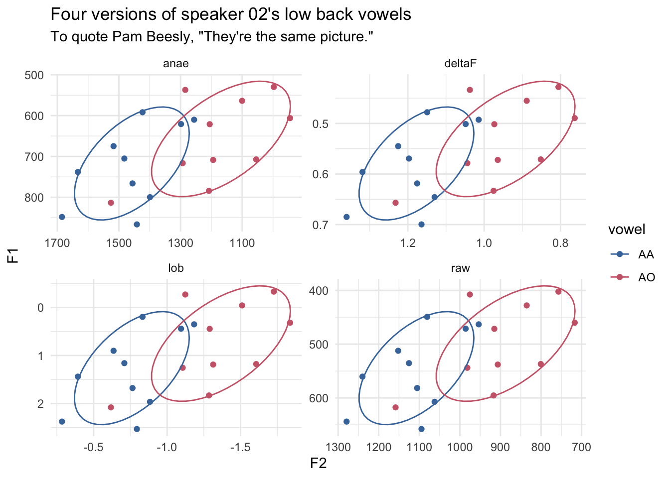
So, as you can see, the plots are virtually identical, other than the scales of the x- and y-axes. This might not be the best illustration of what’s going on because ggplot2 will automatically stretch and center the data, but maybe it works for you?
Conclusion
So there you have it. It doesn’t matter if you calculate pillai scores before or after normalization—at least with the three procedures used here—the results are going to be the same regardless.